QML 101

Quantum Machine Learning (QML) is an emerging and promising research area within quantum computing.

By harnessing quantum phenomena such as superposition and entanglement, QML enables efficient encoding and manipulation of data using multiple qubits. These unique capabilities offer the potential to significantly accelerate machine learning tasks and enhance model expressiveness, especially when working with high-dimensional classical datasets.

As the field continues to develop, QML is expected to play a key role in advancing both quantum and classical machine learning paradigms.

Basics of Quantum Computing

What is a Qubit?

At the heart of quantum computing lies the concept of the quantum bit, or qubit. Unlike a classical bit, which takes on a value of either 0 or 1, a qubit can exist in a superposition of both states simultaneously. This property allows quantum computers to process information in fundamentally different and often more powerful ways than classical systems.

Mathematically, a qubit is described as a unit vector in a two-dimensional complex Hilbert space. Its general state can be written as:

\[\vert \psi \rangle = \alpha \vert 0 \rangle + \beta \vert 1 \rangle,\]

where \(\alpha, \beta \in \mathbb{C}\) and must satisfy the normalization condition:

\[|\alpha|^2 + |\beta|^2 = 1.\]

Here:

\(\vert 0 \rangle\) and \(\vert 1 \rangle\) are the computational basis states,
\(\alpha\) and \(\beta\) are complex probability amplitudes,
and \(\vert \psi \rangle\) is said to be in a superposition of \(\vert 0 \rangle\) and \(\vert 1 \rangle\).

When a measurement is performed in the computational basis, the qubit collapses to one of the basis states with probabilities:

\[P(0) = |\alpha|^2, \quad P(1) = |\beta|^2.\]

To conveniently calculate inner products and probabilities, we also define the bra (the Hermitian conjugate of a ket) as:

\[\langle \psi \vert = \alpha^* \langle 0 \vert + \beta^* \langle 1 \vert,\]

where \(\alpha^*\) and \(\beta^*\) are the complex conjugates of \(\alpha\) and \(\beta\). The inner product (or norm) of the state is then:

\[\langle \psi \vert \psi \rangle = |\alpha|^2 + |\beta|^2 = 1,\]

which confirms the normalization of the quantum state.

This formalism is part of Dirac notation, a standard language for describing quantum states and operations.

More Qubits

When working with multiple qubits, the state of the overall system is represented by the tensor product of the individual qubit states. For example, the state of a two-qubit system can be written as:

\[\begin{split}\begin{align} \vert \psi \rangle &= c_1 \vert 0 \rangle_1 \otimes \vert 0 \rangle_2 + c_2 \vert 0 \rangle_1 \otimes \vert 1 \rangle_2 \\ &\quad + c_3 \vert 1 \rangle_1 \otimes \vert 0 \rangle_2 + c_4 \vert 1 \rangle_1 \otimes \vert 1 \rangle_2 \\ &= c_1 \vert 00 \rangle + c_2 \vert 01 \rangle + c_3 \vert 10 \rangle + c_4 \vert 11 \rangle, \end{align}\end{split}\]

where \(c_1, c_2, c_3, c_4 \in \mathbb{C}\) are complex coefficients satisfying the normalization condition:

\[|c_1|^2 + |c_2|^2 + |c_3|^2 + |c_4|^2 = 1.\]

In many cases, a multi-qubit state can be separated into a product of individual single-qubit states:

\[\vert \psi \rangle = \vert \psi_1 \rangle \otimes \vert \psi_2 \rangle = (\alpha_1 \vert 0 \rangle + \beta_1 \vert 1 \rangle) \otimes (\alpha_2 \vert 0 \rangle + \beta_2 \vert 1 \rangle).\]

However, there exist special quantum states that cannot be written as a tensor product of single-qubit states. These are known as entangled states.

A well-known example is the Bell state:

\[\vert \Phi^+ \rangle = \frac{1}{\sqrt{2}} (\vert 00 \rangle + \vert 11 \rangle),\]

which is entangled because it cannot be decomposed into individual qubit states. In such cases, measuring one qubit instantaneously determines the outcome of the other, regardless of the physical distance between them—a phenomenon that lies at the heart of quantum nonlocality.

Entanglement is a key resource in quantum computing and quantum communication protocols such as quantum teleportation and quantum key distribution.

Quantum Gates and Circuits

Quantum gates are the fundamental operations applied to qubits. They are the quantum analogue of classical logic gates and operate through unitary transformations, which preserve the norm of the quantum state.

A unitary matrix \(U\) satisfies \(U^\dagger U = I\), where \(U^\dagger\) is the conjugate transpose of \(U\), and \(I\) is the identity matrix. Quantum gates can act on one or more qubits at a time.

Common Single-Qubit Gates

These gates act on a single qubit and are represented by \(2 \times 2\) unitary matrices.

Pauli-X (NOT) Gate:

\[\begin{split}X = \begin{bmatrix} 0 & 1 \\ 1 & 0 \end{bmatrix}, \quad X\vert 0 \rangle = \vert 1 \rangle, \quad X\vert 1 \rangle = \vert 0 \rangle\end{split}\]

Pauli-Y Gate:

\[\begin{split}Y = \begin{bmatrix} 0 & -i \\ i & 0 \end{bmatrix}, \quad Y\vert 0 \rangle = i \vert 1 \rangle, \quad Y\vert 1 \rangle = -i \vert 0 \rangle\end{split}\]

Pauli-Z Gate:

\[\begin{split}Z = \begin{bmatrix} 1 & 0 \\ 0 & -1 \end{bmatrix}, \quad Z\vert 0 \rangle = \vert 0 \rangle, \quad Z\vert 1 \rangle = -\vert 1 \rangle\end{split}\]

Hadamard (H) Gate:

\[\begin{split}H = \frac{1}{\sqrt{2}} \begin{bmatrix} 1 & 1 \\ 1 & -1 \end{bmatrix}, \quad H\vert 0 \rangle = \frac{\vert 0 \rangle + \vert 1 \rangle}{\sqrt{2}}, \quad H\vert 1 \rangle = \frac{\vert 0 \rangle - \vert 1 \rangle}{\sqrt{2}}\end{split}\]

Rotation Gates:

These gates perform continuous rotations around the Bloch sphere axes.

\[\begin{split}\begin{aligned} R_x(\theta) &= \cos(\theta/2) I - i \sin(\theta/2) X = \begin{bmatrix} \cos(\theta/2) & -i\sin(\theta/2) \\ -i\sin(\theta/2) & \cos(\theta/2) \end{bmatrix} \\ R_y(\theta) &= \cos(\theta/2) I - i \sin(\theta/2) Y \\ R_z(\theta) &= \begin{bmatrix} e^{-i\theta/2} & 0 \\ 0 & e^{i\theta/2} \end{bmatrix} \end{aligned}\end{split}\]

Common Two-Qubit Gates

Two-qubit gates allow for interaction between qubits and are necessary for creating entanglement.

CNOT (CX) Gate:

A controlled-X gate: flips the target qubit if the control is \(\vert 1 \rangle\).

\[\begin{split}\text{CNOT} = \begin{bmatrix} 1 & 0 & 0 & 0 \\ 0 & 1 & 0 & 0 \\ 0 & 0 & 0 & 1 \\ 0 & 0 & 1 & 0 \end{bmatrix}\end{split}\]
Controlled-Z (CZ) Gate:

Applies a \(Z\) gate to the target qubit only when the control qubit is \(\vert 1 \rangle\).

\[\begin{split}\text{CZ} = \begin{bmatrix} 1 & 0 & 0 & 0 \\ 0 & 1 & 0 & 0 \\ 0 & 0 & 1 & 0 \\ 0 & 0 & 0 & -1 \end{bmatrix}\end{split}\]
SWAP Gate:

Swaps the states of two qubits.

\[\begin{split}\text{SWAP} = \begin{bmatrix} 1 & 0 & 0 & 0 \\ 0 & 0 & 1 & 0 \\ 0 & 1 & 0 & 0 \\ 0 & 0 & 0 & 1 \end{bmatrix}\end{split}\]
Controlled Phase Gate (CPHASE):

Applies a phase shift to the target qubit if the control is \(\vert 1 \rangle\).

\[\begin{split}\text{CPHASE}(\phi) = \begin{bmatrix} 1 & 0 & 0 & 0 \\ 0 & 1 & 0 & 0 \\ 0 & 0 & 1 & 0 \\ 0 & 0 & 0 & e^{i\phi} \end{bmatrix}\end{split}\]
Toffoli Gate (CCX):

A 3-qubit gate. Flips the third (target) qubit if the first two (controls) are both \(\vert 1 \rangle\).

This is a universal gate for classical logic and can implement NAND.

Quantum circuits are constructed by applying a sequence of quantum gates to an initial quantum state. Each line in a quantum circuit diagram represents a qubit, and each gate acts on one or more of those lines.

By combining gates, we can:

Create superposition and entanglement,
Implement quantum algorithms (e.g., Grover’s, Shor’s),
Construct parametrized quantum circuits for variational quantum algorithms (VQAs) such as QVAF-based models.

Quantum circuits form the foundation of all practical quantum algorithms and are programmable through frameworks like Qiskit, Pennylane, and Cirq.

[1]:

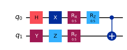
from qiskit import QuantumCircuit

# Create a quantum circuit with 2 qubits
qc = QuantumCircuit(2)

# Apply gates to qubit 0 and qubit 1
qc.h(0)           # Hadamard gate on qubit 0 (creates superposition)
qc.x(0)           # Pauli-X gate (bit-flip) on qubit 0
qc.y(1)           # Pauli-Y gate on qubit 1
qc.z(1)           # Pauli-Z gate on qubit 1
qc.rx(0.5, 0)     # RX rotation by 0.5 radians on qubit 0
qc.ry(0.5, 1)     # RY rotation by 0.5 radians on qubit 1
qc.rz(0.5, 0)     # RZ rotation by 0.5 radians on qubit 0

# Entangling gate: CNOT with control qubit 0 and target qubit 1
qc.cx(0, 1)

# Draw the circuit using matplotlib
qc.draw("mpl")

[1]:

Measurement

Measurement in quantum computing refers to the process of extracting classical information from a quantum state. Upon measurement, a qubit collapses to one of its basis states, with probabilities determined by its quantum amplitudes.

Measurement as an Observable

In quantum mechanics, measurements are associated with Hermitian operators, called observables. A Hermitian operator \(M\) can be expressed in terms of its eigenvalues \(\lambda_i\) and eigenvectors \(\vert m_i \rangle\) as:

\[M = \sum_i \lambda_i \vert m_i \rangle \langle m_i \vert.\]

If a quantum system is in state \(\vert \psi \rangle\), then the probability of obtaining the outcome \(\lambda_i\) (i.e., observing the system in eigenstates \(\vert m_i \rangle\)) is:

\[P(\lambda_i) = |\langle m_i \vert \psi \rangle|^2.\]

Measurement as a Projection

To compute this probability, we often interpret measurement as a projection using the measurement operator \(M_i = \vert m_i \rangle \langle m_i \vert\). Then:

\[P(\lambda_i) = \langle \psi \vert M_i^\dagger M_i \vert \psi \rangle = \langle \psi \vert M_i \vert \psi \rangle = |\langle m_i \vert \psi \rangle|^2,\]

where \(M_i^\dagger = M_i\) because \(M_i\) is Hermitian and \(M_i^2 = M_i\) because it’s a projector.

Measurement in the Computational Basis

In practice, quantum computers typically measure qubits in the computational basis, which corresponds to the eigenstates of the Pauli-Z operator:

\(\vert 0 \rangle\) with eigenvalue \(+1\),
\(\vert 1 \rangle\) with eigenvalue \(-1\).

Given a single-qubit state:

\[\vert \psi \rangle = \alpha \vert 0 \rangle + \beta \vert 1 \rangle,\]

the expected value of the Pauli-Z measurement is:

\[\langle Z \rangle = \langle \psi \vert Z \vert \psi \rangle = |\alpha|^2 - |\beta|^2.\]

This expectation value is useful in variational quantum algorithms, where observables are evaluated to guide optimization.

⚠️ Note: Measurement irreversibly collapses the quantum state. Once measured, the quantum system is no longer in a superposition but in the observed basis state.

[2]:

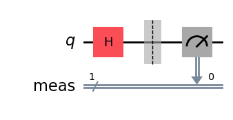
qc = QuantumCircuit(1)
qc.h(0)
qc.measure_all()
qc.draw("mpl")

[2]:

Variational Quantum Algorithms (VQA)

Variational Quantum Algorithms (VQAs) are a class of hybrid quantum-classical algorithms that combine the power of quantum processors with classical optimization techniques. They have shown great promise for tackling optimization problems, quantum simulation, and machine learning tasks.

The core idea behind VQAs is to use a parameterized quantum circuit (also called an ansatz) to prepare quantum states, and iteratively optimize the circuit parameters using classical algorithms.

The typical workflow of a VQA involves the following steps:

Data Encoding:

Classical data is encoded into quantum states through specially designed quantum circuits. Efficient encoding is essential in quantum machine learning to represent complex classical data in a quantum system.
Variational Circuit (Parameterized Unitaries):

A quantum circuit composed of gates with adjustable parameters (e.g., rotation angles) is applied. This circuit transforms the initial quantum state into a parameter-dependent state that captures features of the data or the problem.
Measurement:

The quantum state is measured to extract classical information. Measurement outcomes are used to compute a cost function (or objective function), which quantifies how well the current parameters solve the problem.
Classical Optimization:

Classical optimization algorithms (such as gradient descent, COBYLA, or SPSA) update the circuit parameters to minimize or maximize the cost function. This feedback loop continues until convergence or a stopping criterion is met.

VQAs are flexible and can be tailored for various applications such as:

Quantum Approximate Optimization Algorithm (QAOA) for combinatorial optimization
Variational Quantum Eigensolver (VQE) for estimating ground-state energies in chemistry
Quantum Neural Networks for machine learning

The hybrid nature of VQAs makes them particularly suitable for near-term noisy quantum devices, leveraging classical computation to mitigate hardware limitations.

Quantum Kernel Methods

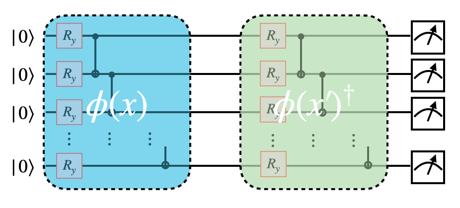
Quantum Kernel Methods are quantum machine learning algorithms inspired by classical kernel methods such as Support Vector Machines (SVMs). They rely on the quantum feature map — a parameterized quantum circuit that embeds classical input data into a high-dimensional Hilbert space.

The key idea is to compute the kernel function between data points as the inner product of quantum states:

\[k(x, x') = |\langle \phi(x) \vert \phi(x') \rangle|^2\]

where \(\vert \phi(x) \rangle\) is the quantum state that encodes the classical input \(x\).

Quantum kernel methods offer potential quantum advantage by exploiting Hilbert spaces too large to simulate classically, enabling powerful nonlinear classification with linear algorithms.

Workflow of a Quantum Kernel Method

Feature Map (Encoding Circuit): Encode classical data \(x\) into a quantum state \(\vert \phi(x) \rangle\) using a quantum circuit.
Compute Kernel Matrix: For a dataset \(\{x_i\}\), compute \(k(x_i, x_j)\) using quantum overlaps between states.
Classical Algorithm: Use a classical kernel method (e.g., SVM) with the quantum kernel matrix for classification or regression.

Data Re-Uploading Circuits

Data re-uploading is a strategy used in parameterized quantum circuits where the input data is encoded multiple times throughout the layers of a variational quantum circuit. This technique enhances the expressivity of quantum models and is especially useful in quantum neural networks (QNNs).

In contrast to basic quantum models that encode the data once at the beginning, re-uploading introduces classical input features at multiple points in the circuit. This allows the circuit to model more complex, nonlinear functions—similar to the depth and recurrence seen in classical neural networks.

Why Re-Upload Data?

Quantum circuits are often constrained in depth due to hardware noise and decoherence. Re-uploading helps:

Compensate for shallow circuits by increasing expressivity.
Introduce nonlinearity through the interplay of data and trainable parameters.
Enable better generalization and function approximation in quantum models.

General Structure

A typical data re-uploading circuit follows this pattern:

Apply data-encoding gates (e.g., \(R_x(x), R_y(x), R_z(x)\)).
Apply trainable gates (e.g., \(R_y(\theta), R_z(\theta)\)).
Repeat steps 1 and 2 for multiple layers.